How to Match Data in Excel from Two Worksheets

Did you know? Coefficient eliminates the need to export data manually and rebuild stale dashboards. Get started by pulling live data into pre-built Sheets dashboards.

Want to compare data between two Excel worksheets? You’re in the right place!

This guide shows you how to match and link data from different sheets in Excel. You’ll learn useful functions and techniques to find and connect related information.

Data Matching in Excel: Understanding the Basics

Data matching in Excel refers to the process of identifying and linking corresponding records from two or more data sources, such as worksheets or tables. This is a common task for data analysts, finance professionals, and anyone who needs to consolidate and analyze data from different sources.

Accurate data matching enables you to:

Combine data from multiple sources for comprehensive analysis
Identify relationships and patterns across your data
Eliminate duplicate records and ensure data integrity
Streamline reporting and decision-making processes

Match Data in Excel from Two Worksheets: 3 Methods and Tutorial

Method 1: Using VLOOKUP to Match Data in Excel

One of the most commonly used functions for data matching in Excel is VLOOKUP. This powerful function allows you to look up and retrieve data from a table or range, based on a value in the first column of that table or range.

Here’s a step-by-step guide on how to use VLOOKUP for data matching:

Identify the data sources: Ensure that the data you want to match is organized in a tabular format, with a unique identifier (such as a customer ID or product code) in the first column.
Arrange the data: Ensure that the data you want to match is organized in a tabular format, with a unique identifier (such as a customer ID or product code) in the first column.
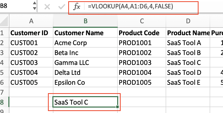
Construct the VLOOKUP formula: The basic VLOOKUP formula is: =VLOOKUP(lookup_value, table_array, col_index_num, [range_lookup])
- lookup_value: The value you want to look up (e.g., a customer ID or product code)
- table_array: The range of cells where the lookup data is located
- col_index_num: The column number within the table_array that contains the value you want to return
- [range_lookup]: A logical value that specifies whether you want an exact match (FALSE) or an approximate match (TRUE)

Troubleshoot common VLOOKUP issues: Be aware of potential pitfalls, such as case sensitivity, data type mismatches, and the importance of ensuring that the lookup value is in the first column of the table_array.

Method 2: Using INDEX MATCH for Data Matching

While VLOOKUP is a widely used function, it has some limitations, such as the requirement for the lookup value to be in the first column of the table_array. To overcome these limitations, you can use the combination of the INDEX and MATCH functions, known as INDEX MATCH.

Here’s how to use INDEX MATCH for data matching:

Identify the data sources: Ensure that the data you want to match is organized in a tabular format, with a unique identifier (such as a customer ID or product code) in any column.
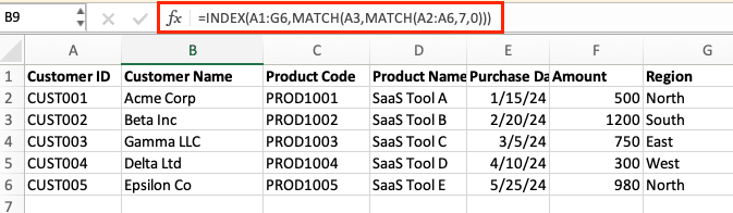
Construct the INDEX MATCH formula: The basic INDEX MATCH formula is: =INDEX(return_range, MATCH(lookup_value,lookup_range, [match_type]))
- return_range: The range of cells that contains the values you want to return
- lookup_value: The value you want to look up (e.g., a customer ID or product code)
- lookup_range: The range of cells that contains the lookup values
- [match_type]: A number that specifies the type of match you want (1 for exact match, 0 for exact match, -1 for approximate match)

Understand the advantages of INDEX MATCH: INDEX MATCH offers more flexibility than VLOOKUP, as it allows you to look up values in any column of the table, not just the first column. It also handles cases where the lookup value is not in the first column more effectively.

Method 3: Combining Functions for Advanced Matching

When dealing with complex data matching scenarios, you can take your Excel skills to the next level by combining powerful functions like VLOOKUP, INDEX MATCH, and IFERROR. This approach allows you to handle more intricate data relationships and achieve greater accuracy in your matching process.

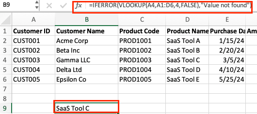
Let’s start by exploring how to use the VLOOKUP and IFERROR functions together. The IFERROR function can help you gracefully handle situations where the VLOOKUP function returns an error, such as when a lookup value is not found.

By nesting these two functions, you can create a robust solution that provides a default value or message rather than displaying an error when the lookup fails.

=IFERROR(VLOOKUP(lookup_value, range, column_index, [range_lookup]), “Value not found”)

Highlighting Differences Between Two Worksheets

Comparing data across multiple worksheets can be tedious, but Excel’s conditional formatting feature can make this process much more efficient. Conditional formatting allows you to quickly identify and highlight the differences between two worksheets, making it easier to spot discrepancies and ensure data integrity.

Coefficient Excel Google Sheets Connectors

Try the Free Spreadsheet Extension Over 425,000 Pros Are Raving About

Stop exporting data manually. Sync data from your business systems into Google Sheets or Excel with Coefficient and set it on a refresh schedule.

Here’s a step-by-step guide to highlighting differences using conditional formatting:

Prepare your data: Ensure that the data in both worksheets is formatted consistently, with matching column headers and data types.
Create a new column: Add a new column to one of the worksheets, where you’ll perform the comparison.
Use the VLOOKUP function: In the new column, use the VLOOKUP function to look up the corresponding value from the other worksheet. If the value is not found, the VLOOKUP function will return an error.
Apply conditional formatting: Select the column with the VLOOKUP results and apply conditional formatting. Set the formatting rule to highlight cells with errors (e.g., use a red fill color or a bold font).

By following this process, you can quickly identify any mismatched or missing data between the two worksheets, making it easier to investigate and resolve any discrepancies.

Troubleshooting Common Issues

Data matching in Excel is not without its challenges, and it’s important to be prepared to address common issues that may arise. Let’s explore some of the most common problems and discuss effective solutions.

Mismatched Data Types: If the data types in your source and target worksheets don’t match, the lookup functions may not work as expected. For example, if one worksheet has a numeric value and the other has the same value as text, the VLOOKUP function may not be able to find the match. To resolve this, you can use the TRIM and VALUE functions to ensure consistent data types.
Missing Values: When dealing with incomplete data, you may encounter situations where the lookup function can’t find a match. This can lead to errors or unexpected results. To handle missing values, you can use the IFERROR function, as mentioned earlier, to provide a default value or message when a lookup fails.
Formula Errors: Errors in your formulas can cause unexpected results and make data matching a frustrating experience. Always double-check your formulas, and consider using the Formula Auditing tools in Excel to help identify and fix any issues.
Performance Concerns: As the size of your datasets grows, the performance of your data matching formulas may start to suffer. To optimize performance, you can try techniques like using structured references, minimizing nested functions, and leveraging Excel’s built-in data analysis tools, such as Power Query.

By being aware of these common issues and having a toolbox of solutions at your disposal, you’ll be better equipped to tackle any data matching challenges that come your way.

Mastering Data Matching in Excel

You now know how to match data between two Excel worksheets. These methods help you connect and compare information across your spreadsheets. Remember to choose the right technique based on your data structure.

Want to make data matching even easier? Try Coefficient to automatically sync data from different sources into your Excel sheets, saving you time on manual matching.

SERP Title: Mastering Data Matching in Excel: Advanced Techniques and Best Practices Meta Description: Discover advanced data matching methods in Excel, including combining functions, highlighting differences, and troubleshooting common issues. Improve your data management skills with this comprehensive guide.

Sync Live Data into Excel

Connect Excel to your business systems, import your data, and set it on a refresh schedule.